For the purposes of this activity we’ll use data from the 1994 census (there are fewer variables than the proteomics data and sometimes a little variety is nice).
Action
On the group workstation at your table, have one person open a new R script and copy-paste the chunk below to load the data.
You will not need to store a copy of your work (unless you want to) – so the script is just to be able to perform some simple calculations during class.
First, draw a sample with replacement from the observations. This is known as a bootstrap sample. We’ll keep this relatively small to simplify matters.
Action
Draw a bootstrap sample
Copy the code chunk below and execute once.
# resample datacensus_boot <- census %>%sample_n(size =200, replace = T)
You will build your tree using this data.
Step 2: select predictors at random
Next draw a set of predictors at random. We’ll also keep this set small so that you can develop the tree ‘by hand’.
Action
Select two random predictors
Copy and paste the code chunk below into your script and execute once without modification.
# retrieve column namespossible_predictors <- census %>%select(-income) %>%colnames()# grab 2 columns at randompredictors <-sample(possible_predictors,size =2, replace = F)# select these columns from the bootstrap sampletrain <- census_boot %>%select(c(income, any_of(predictors)))
You will build your tree using only these predictors from the bootstrap sample as training data.
Step 3a: find your first split
Now your job is to choose exactly one of the predictors to make a binary split of the data.
for categorical variables, determine which categories you will classify as high-income vs. low-income
for continuous variables, choose a cutoff value so that any observation greater/less than the cutoff is classified as a high/low (or vice-versa) earner
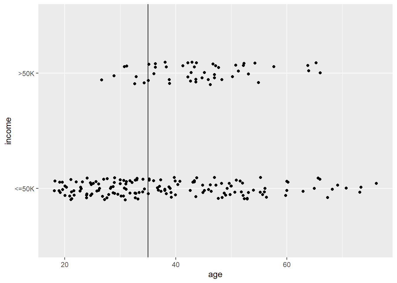
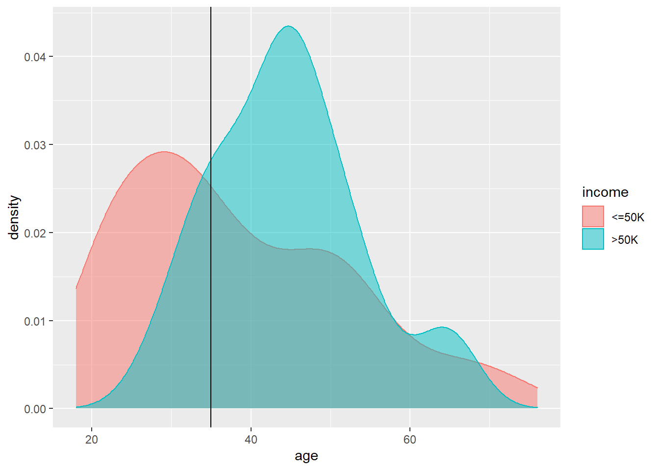
You do not need to make quantitatively rigorous choices. Try to make a choice that you think is reasonable, but don’t agonize over it. The code below might help you decide which variable to use and how to make the split: use it to inspect each of the two variables and decide which one better distinguishes the income groups.
# comment out -- don't overwrite your bootstrap sample!census_boot <- census %>%sample_n(size =200, replace = T)# for continuous variablescensus_boot %>%ggplot(aes(x = age, # replace with predictor name y = income)) +geom_jitter(height =0.1) +geom_vline(xintercept =35) # adjust cutoff
# pick out categories that are majority high incomehighinc_categories <- census_boot %>%group_by(workclass, # replace with predictor name income) %>%count() %>%spread(income, n) %>%mutate_all(~replace_na(.x, 0)) %>%mutate(high.inc =`<=50K`<`>50K`) %>%filter(high.inc == T) %>%pull(workclass) # replace with predictor name
Action
Make your first split
Choose whichever of the two predictors you think best distinguishes the high income and low income groups.
Find a cutoff value if the variable is continuous, or the categories that you will classify as high income if the variable is categorical.
If categorical, store a vector of the category names that are classified as high income (see code above). If continuous, store the cutoff value.
Write down the rule.
Step 3b: find your second split
Now filter the data to just those rows classified as (but not necessarily actually) high income based on your first split.
# continuous case -- examplecutoff <-35census_boot_sub <- census_boot %>%filter(age > cutoff)# categorical case -- examplecensus_boot_sub <- census_boot %>%filter(workclass %in% highinc_categories)
Action
Find a second split
Repeat step 3a but with the filtered data census_boot_sub instead of the full bootstrap sample.
Write down the rule.
Step 4: draw the tree
We could in theory keep creating binary splits until all observations are correctly classified. However, since we’re doing this by hand and just for illustration purposes, we’ll stop after two splits – it’ll be more of a sapling than a fully grown tree.
Action
Make a diagram
Draw your tree on your group’s whiteboard. It should have just one ‘root’ node and just three ‘leaf’ nodes.
Classifying a new observation
Use your tree to determine how to classify the following observation:
census %>%sample_n(size =1) %>%t() %>% knitr::kable()
age
56
workclass
Private
education
HS-grad
marital_status
Divorced
occupation
Adm-clerical
relationship
Other-relative
race
Amer-Indian-Eskimo
sex
Female
capital_gain
0
capital_loss
0
hours_per_week
35
native_country
United-States
income
<=50K
Algorithmic considerations
You just did a loose version of what’s known as recursive partitioning – repeatedly splitting the data. That’s a specific method of constructing a tree.
How did you decide which of your two variables to use? Could you write code to make the same choice automatically? This, it turns out, is the main challenge in fully automating the process. The recursive partitioning algorithm requires two things:
a criterion by which one split is considered ‘better’ than another
a stopping rule
It is fairly simple to compute the best cutoff (or categorical mapping) for a given predictor – one can do a brute-force search for the split that minimizes misclassifications. However, when there are many possible variables to split on, a criterion is needed to determine the best choice. You can read about how this is done in MDSR 11.1.1.