Training neural networks

Pre-lab activity

Please complete this activity before arriving at your section meeting. It should only take you about 15 minutes.

Python installation

We will use packages that interface to python from R to train neural networks in this lab. For this a current python installation is needed.

Select the download appropriate for your operating system here and follow installation instructions.

Keras and Tensorflow

Open RStudio and execute the following commands in the console. You should have already installed keras with other packages in the first lab; however, if library(keras) returns an error execute install.packages('keras') and then try again. This will install Tensorflow (for python) in a manner suitable for use in R, along with a few other packages.

library(keras)
install_keras()

To confirm the installation worked, try:

library(tensorflow)
tf$constant('Hello world')

tf.Tensor(b'Hello world', shape=(), dtype=string)

You may see a long message related to CUDA libraries in addition to the output shown above, but if you see this output at the end, your installation was successful.

If you did not see the expected output, try configuring a virtual environment for the installation explicitly as shown here.

If you are unable to troubleshoot after a short period of time, partner with a classmate for the lab activity and then ask for help from course staff.

Lab activity

Setup

ImportantAction

Setup

Open a new script for this lab, copy-paste the code chunk below at the top of the script, and execute once.

# packages
library(tidyverse)
library(tidymodels)
library(tidytext)
library(keras)
library(tensorflow)

# data location
url <- 'https://raw.githubusercontent.com/pstat197/pstat197a/main/materials/labs/lab6-nn/data/claims-clean.csv'

# read in data
clean <- read_csv(url)

Now partition the data into training and test sets.

ImportantAction

Data partitioning

1. Copy the code chunk below into your script but do not run the resulting lines.
2. Coordinate with your neighbor: choose a new RNG seed and split proportion and input the same values in each of your scripts.
3. Execute lines to partition the data.

# partition
set.seed(110325)
partitions <- clean %>%
  mutate(text_clean = str_trim(text_clean)) %>%
  filter(str_length(text_clean) > 5) %>%
  initial_split(prop = 0.8)

Now use the code chunk below to preprocess the training partition into a TF-IDF document term matrix (DTM), as before.

train_dtm <- training(partitions) %>%
  unnest_tokens(output = 'token', 
                input = text_clean) %>%
  group_by(.id, bclass) %>%
  count(token) %>%
  bind_tf_idf(term = token, 
              document = .id, 
              n = n) %>%
  pivot_wider(id_cols = c(.id, bclass), 
              names_from = token, 
              values_from = tf_idf,
              values_fill = 0) %>%
  ungroup()

Logistic regression as NN

To get a feel for keras, first we’ll fit a logistic regression model.

Recall that in class it was mentioned that standard statistical models can be described by neural networks with no hidden layers; along these lines, standard statistical models can also be fit using optimization routines for neural network training.

Use the code chunk below to get the TF-IDF values for the (alphabetically) first ten tokens. We’ll use these as predictors.

# extract first ten features
x_train <- train_dtm %>%
  ungroup() %>%
  select(-.id, -bclass) %>%
  select(1:10) %>%
  as.matrix()

# extract labels and coerce to binary
y_train <- train_dtm %>% 
  pull(bclass) %>%
  factor() %>%
  as.numeric() - 1

This is purely for illustration purposes; any model using these variables should not perform well at all because ten tokens won’t contain much information about the classes.

To use keras, we’ll go through a few steps that are generally not done separately for fitting statistical models:

1. Model specification, i.e.,defining an architecture

2. Model configuration, i.e., specifying a loss function and fitting method

3. Model training, i.e., computing estimates for the parameters

Model specification

Model architecture is defined layer-by-layer. Keras has some preconfigured model types: for feedforward networks, use keras_model_sequential() .

# specify model type
model <- keras_model_sequential(input_shape = 10)

The input_shape argument specifies the number of units for the input layer – in other words, the number of predictors.

At this stage, the model is just scaffolding:

summary(model)

Model: "sequential"
________________________________________________________________________________
 Layer (type)                       Output Shape                    Param #     
================================================================================
================================================================================
Total params: 0 (0.00 Byte)
Trainable params: 0 (0.00 Byte)
Non-trainable params: 0 (0.00 Byte)
________________________________________________________________________________

Now layers can be added one-by-one. For now we’ll just add an output layer – one unit. layer_dense will specify that the previous layer is fully-connected to the added layer.

# add output layer
model <- model %>% layer_dense(1) 

The model summary now shows the output layer.

summary(model)

Model: "sequential"
________________________________________________________________________________
 Layer (type)                       Output Shape                    Param #     
================================================================================
 dense (Dense)                      (None, 1)                       11          
================================================================================
Total params: 11 (44.00 Byte)
Trainable params: 11 (44.00 Byte)
Non-trainable params: 0 (0.00 Byte)
________________________________________________________________________________

Lastly, we’ll add a sigmoid activation function:

model <- model %>% 
  layer_activation(activation = 'sigmoid')

Since there is no hidden layer, our model is

\[ \begin{aligned} \mathbb{E}Y &= \frac{1}{1 + \exp\{-T\}} \\ T &= X\beta \end{aligned} \]

Notice that this is the logistic regression model (without the distributional assumption).

Model configuration

Configuring a keras model consists in equipping it with a loss and an optimization method. Optionally, metrics that you’d like computed at each training epoch can be included.

model %>% compile(
  loss = 'binary_crossentropy',
  optimizer = tf$keras$optimizers$legacy$SGD(),
  metrics = 'binary_accuracy'
)

This says that to train the model, we’ll minimize binary cross-entropy on the training data using stochastic gradient descent.

To train for 10 epochs, pipe the model into fit() and supply the training data. Note that the training data must be numeric, not a data frame.

history <- model %>%
  fit(x = x_train, 
      y = y_train,
      epochs = 10)

Epoch 1/10
14/14 - 9s - loss: 0.6932 - binary_accuracy: 0.4955 - 9s/epoch - 610ms/step
Epoch 2/10
14/14 - 0s - loss: 0.6932 - binary_accuracy: 0.5226 - 40ms/epoch - 3ms/step
Epoch 3/10
14/14 - 0s - loss: 0.6932 - binary_accuracy: 0.5158 - 14ms/epoch - 982us/step
Epoch 4/10
14/14 - 0s - loss: 0.6932 - binary_accuracy: 0.5136 - 12ms/epoch - 853us/step
Epoch 5/10
14/14 - 0s - loss: 0.6932 - binary_accuracy: 0.5113 - 11ms/epoch - 803us/step
Epoch 6/10
14/14 - 0s - loss: 0.6931 - binary_accuracy: 0.5158 - 11ms/epoch - 761us/step
Epoch 7/10
14/14 - 0s - loss: 0.6932 - binary_accuracy: 0.5113 - 10ms/epoch - 734us/step
Epoch 8/10
14/14 - 0s - loss: 0.6931 - binary_accuracy: 0.5090 - 10ms/epoch - 695us/step
Epoch 9/10
14/14 - 0s - loss: 0.6931 - binary_accuracy: 0.5113 - 9ms/epoch - 665us/step
Epoch 10/10
14/14 - 0s - loss: 0.6931 - binary_accuracy: 0.5090 - 11ms/epoch - 783us/step

The following commands will retrieve weights, evaluated loss ans specified metrics, and predictions.

# retrieve weights
keras::get_weights(model)

[[1]]
            [,1]
 [1,] -0.1005378
 [2,] -0.3915481
 [3,]  0.3347541
 [4,]  0.5459515
 [5,] -0.7315308
 [6,] -0.5480485
 [7,] -0.2511801
 [8,]  0.1062602
 [9,] -0.1980933
[10,] -0.1905470

[[2]]
[1] -0.01072753

# evaluate on specified data
evaluate(model, x_train, y_train)

14/14 - 0s - loss: 0.6931 - binary_accuracy: 0.5090 - 330ms/epoch - 24ms/step

           loss binary_accuracy 
      0.6930834       0.5090498 

# compute predictions
model(x_train) %>% head()

tf.Tensor(
[[0.49550927]
 [0.49707136]
 [0.49709657]
 [0.49679318]
 [0.49627778]
 [0.49731815]], shape=(6, 1), dtype=float32)

ImportantAction

Check your understanding

Discuss with your neighbor:

1. How many parameters does this model have?
2. Do the number of parameters match your expectations?
3. Why will the parameter estimates not match the result of glm() ?
4. Would further training epochs improve the performance?

Single-layer network

Now that you have a sense of the basic keras syntax and model specification/configuration/training procedure, we can train a proper network with one (or more!) hidden layers.

First coerce the DTM into the format needed for training.

# store full DTM as a matrix
x_train <- train_dtm %>%
  select(-bclass, -.id) %>%
  as.matrix()

Now configure a model with one hidden layer having 10 units. Notice that the architecture can be defined by one sequence of pipes rather than stepwise as before.

model <- keras_model_sequential(input_shape = ncol(x_train)) %>%
  layer_dense(10) %>%
  layer_dense(1) %>%
  layer_activation(activation = 'sigmoid')

summary(model)

Model: "sequential_1"
________________________________________________________________________________
 Layer (type)                       Output Shape                    Param #     
================================================================================
 dense_2 (Dense)                    (None, 10)                      167410      
 dense_1 (Dense)                    (None, 1)                       11          
 activation_1 (Activation)          (None, 1)                       0           
================================================================================
Total params: 167421 (653.99 KB)
Trainable params: 167421 (653.99 KB)
Non-trainable params: 0 (0.00 Byte)
________________________________________________________________________________

Notice the number of parameters. (Does this match your expectation?) Configure the model:

model %>%
  compile(
    loss = 'binary_crossentropy',
    optimizer = tf$keras$optimizers$legacy$SGD(),
    metrics = 'binary_accuracy'
  )

And finally, train:

history <- model %>%
  fit(x = x_train,
      y = y_train,
      epochs = 50)

Epoch 1/50
14/14 - 1s - loss: 0.6931 - binary_accuracy: 0.5090 - 556ms/epoch - 40ms/step
Epoch 2/50
14/14 - 0s - loss: 0.6930 - binary_accuracy: 0.5000 - 76ms/epoch - 5ms/step
Epoch 3/50
14/14 - 0s - loss: 0.6929 - binary_accuracy: 0.5113 - 74ms/epoch - 5ms/step
Epoch 4/50
14/14 - 0s - loss: 0.6929 - binary_accuracy: 0.5068 - 53ms/epoch - 4ms/step
Epoch 5/50
14/14 - 0s - loss: 0.6929 - binary_accuracy: 0.5045 - 41ms/epoch - 3ms/step
Epoch 6/50
14/14 - 0s - loss: 0.6928 - binary_accuracy: 0.5045 - 31ms/epoch - 2ms/step
Epoch 7/50
14/14 - 0s - loss: 0.6927 - binary_accuracy: 0.5045 - 34ms/epoch - 2ms/step
Epoch 8/50
14/14 - 0s - loss: 0.6926 - binary_accuracy: 0.5090 - 24ms/epoch - 2ms/step
Epoch 9/50
14/14 - 0s - loss: 0.6925 - binary_accuracy: 0.5068 - 28ms/epoch - 2ms/step
Epoch 10/50
14/14 - 0s - loss: 0.6925 - binary_accuracy: 0.5045 - 26ms/epoch - 2ms/step
Epoch 11/50
14/14 - 0s - loss: 0.6925 - binary_accuracy: 0.5045 - 25ms/epoch - 2ms/step
Epoch 12/50
14/14 - 0s - loss: 0.6923 - binary_accuracy: 0.5068 - 23ms/epoch - 2ms/step
Epoch 13/50
14/14 - 0s - loss: 0.6923 - binary_accuracy: 0.5045 - 24ms/epoch - 2ms/step
Epoch 14/50
14/14 - 0s - loss: 0.6922 - binary_accuracy: 0.5090 - 25ms/epoch - 2ms/step
Epoch 15/50
14/14 - 0s - loss: 0.6922 - binary_accuracy: 0.5068 - 30ms/epoch - 2ms/step
Epoch 16/50
14/14 - 0s - loss: 0.6921 - binary_accuracy: 0.5090 - 18ms/epoch - 1ms/step
Epoch 17/50
14/14 - 0s - loss: 0.6922 - binary_accuracy: 0.5113 - 18ms/epoch - 1ms/step
Epoch 18/50
14/14 - 0s - loss: 0.6921 - binary_accuracy: 0.5068 - 17ms/epoch - 1ms/step
Epoch 19/50
14/14 - 0s - loss: 0.6920 - binary_accuracy: 0.5090 - 17ms/epoch - 1ms/step
Epoch 20/50
14/14 - 0s - loss: 0.6919 - binary_accuracy: 0.5113 - 20ms/epoch - 1ms/step
Epoch 21/50
14/14 - 0s - loss: 0.6919 - binary_accuracy: 0.5090 - 23ms/epoch - 2ms/step
Epoch 22/50
14/14 - 0s - loss: 0.6918 - binary_accuracy: 0.5068 - 23ms/epoch - 2ms/step
Epoch 23/50
14/14 - 0s - loss: 0.6918 - binary_accuracy: 0.5113 - 22ms/epoch - 2ms/step
Epoch 24/50
14/14 - 0s - loss: 0.6917 - binary_accuracy: 0.5113 - 19ms/epoch - 1ms/step
Epoch 25/50
14/14 - 0s - loss: 0.6917 - binary_accuracy: 0.5113 - 19ms/epoch - 1ms/step
Epoch 26/50
14/14 - 0s - loss: 0.6915 - binary_accuracy: 0.5113 - 19ms/epoch - 1ms/step
Epoch 27/50
14/14 - 0s - loss: 0.6915 - binary_accuracy: 0.5113 - 21ms/epoch - 2ms/step
Epoch 28/50
14/14 - 0s - loss: 0.6914 - binary_accuracy: 0.5113 - 23ms/epoch - 2ms/step
Epoch 29/50
14/14 - 0s - loss: 0.6914 - binary_accuracy: 0.5113 - 22ms/epoch - 2ms/step
Epoch 30/50
14/14 - 0s - loss: 0.6913 - binary_accuracy: 0.5113 - 23ms/epoch - 2ms/step
Epoch 31/50
14/14 - 0s - loss: 0.6912 - binary_accuracy: 0.5113 - 23ms/epoch - 2ms/step
Epoch 32/50
14/14 - 0s - loss: 0.6913 - binary_accuracy: 0.5113 - 24ms/epoch - 2ms/step
Epoch 33/50
14/14 - 0s - loss: 0.6912 - binary_accuracy: 0.5113 - 29ms/epoch - 2ms/step
Epoch 34/50
14/14 - 0s - loss: 0.6911 - binary_accuracy: 0.5113 - 28ms/epoch - 2ms/step
Epoch 35/50
14/14 - 0s - loss: 0.6910 - binary_accuracy: 0.5113 - 23ms/epoch - 2ms/step
Epoch 36/50
14/14 - 0s - loss: 0.6911 - binary_accuracy: 0.5068 - 31ms/epoch - 2ms/step
Epoch 37/50
14/14 - 0s - loss: 0.6909 - binary_accuracy: 0.5204 - 34ms/epoch - 2ms/step
Epoch 38/50
14/14 - 0s - loss: 0.6908 - binary_accuracy: 0.5181 - 33ms/epoch - 2ms/step
Epoch 39/50
14/14 - 0s - loss: 0.6908 - binary_accuracy: 0.5294 - 34ms/epoch - 2ms/step
Epoch 40/50
14/14 - 0s - loss: 0.6907 - binary_accuracy: 0.5271 - 35ms/epoch - 3ms/step
Epoch 41/50
14/14 - 0s - loss: 0.6907 - binary_accuracy: 0.5204 - 25ms/epoch - 2ms/step
Epoch 42/50
14/14 - 0s - loss: 0.6906 - binary_accuracy: 0.5294 - 23ms/epoch - 2ms/step
Epoch 43/50
14/14 - 0s - loss: 0.6905 - binary_accuracy: 0.5271 - 20ms/epoch - 1ms/step
Epoch 44/50
14/14 - 0s - loss: 0.6905 - binary_accuracy: 0.5294 - 20ms/epoch - 1ms/step
Epoch 45/50
14/14 - 0s - loss: 0.6904 - binary_accuracy: 0.5294 - 21ms/epoch - 1ms/step
Epoch 46/50
14/14 - 0s - loss: 0.6904 - binary_accuracy: 0.5294 - 20ms/epoch - 1ms/step
Epoch 47/50
14/14 - 0s - loss: 0.6903 - binary_accuracy: 0.5294 - 19ms/epoch - 1ms/step
Epoch 48/50
14/14 - 0s - loss: 0.6903 - binary_accuracy: 0.5294 - 19ms/epoch - 1ms/step
Epoch 49/50
14/14 - 0s - loss: 0.6902 - binary_accuracy: 0.5294 - 20ms/epoch - 1ms/step
Epoch 50/50
14/14 - 0s - loss: 0.6902 - binary_accuracy: 0.5294 - 18ms/epoch - 1ms/step

plot(history)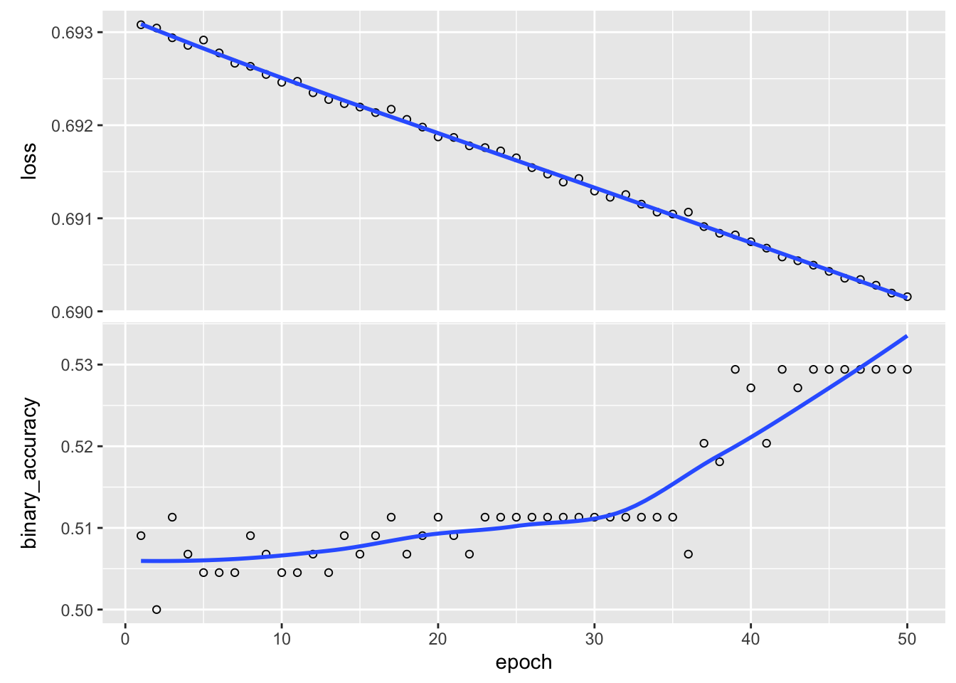

Notice that even after 50 epochs the results are still quite poor. As mentioned in class, the choice of optimization method can have a big impact on the quality of estimates. If we train the model instead using Adam, good accuracy is achieved after just a few epochs:

# change the optimizer
model %>%
  compile(
    loss = 'binary_crossentropy',
    optimizer = 'adam',
    metrics = 'binary_accuracy'
  )

# re-train
history <- model %>%
  fit(x = x_train,
      y = y_train,
      epochs = 10)

Epoch 1/10
14/14 - 2s - loss: 0.6876 - binary_accuracy: 0.5294 - 2s/epoch - 149ms/step
Epoch 2/10
14/14 - 0s - loss: 0.6734 - binary_accuracy: 0.6312 - 19ms/epoch - 1ms/step
Epoch 3/10
14/14 - 0s - loss: 0.6586 - binary_accuracy: 0.8394 - 18ms/epoch - 1ms/step
Epoch 4/10
14/14 - 0s - loss: 0.6426 - binary_accuracy: 0.9050 - 18ms/epoch - 1ms/step
Epoch 5/10
14/14 - 0s - loss: 0.6257 - binary_accuracy: 0.9186 - 18ms/epoch - 1ms/step
Epoch 6/10
14/14 - 0s - loss: 0.6070 - binary_accuracy: 0.9367 - 18ms/epoch - 1ms/step
Epoch 7/10
14/14 - 0s - loss: 0.5877 - binary_accuracy: 0.9502 - 17ms/epoch - 1ms/step
Epoch 8/10
14/14 - 0s - loss: 0.5675 - binary_accuracy: 0.9502 - 17ms/epoch - 1ms/step
Epoch 9/10
14/14 - 0s - loss: 0.5465 - binary_accuracy: 0.9548 - 17ms/epoch - 1ms/step
Epoch 10/10
14/14 - 0s - loss: 0.5252 - binary_accuracy: 0.9548 - 17ms/epoch - 1ms/step

plot(history)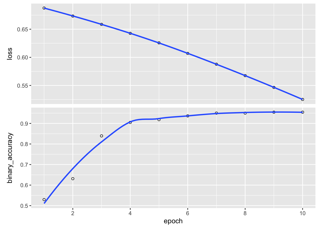

Validation data

Often training data are sub-partitioned into training and ‘validation’ sets. The validation set can be used to provide a soft estimate of accuracy during training.

This provides one strategy to avoid overfitting – the practitioner should only train as long as validation accuracy continues to increase.

Keras makes that easy by supplying an extra argument to fit(). The code chunk below trains for longer and uses 20% of the training data for validation. You should see that the training accuracy gets quite high, but the validation accuracy plateaus around 80%.

# redefine model
model <- keras_model_sequential(input_shape = ncol(x_train)) %>%
  layer_dense(10) %>%
  layer_dense(1) %>%
  layer_activation(activation = 'sigmoid')

model %>%
  compile(
    loss = 'binary_crossentropy',
    optimizer = 'adam',
    metrics = 'binary_accuracy'
  )

# train with validation split
history <- model %>%
  fit(x = x_train,
      y = y_train,
      epochs = 20,
      validation_split = 0.2)

Epoch 1/20
12/12 - 1s - loss: 0.6913 - binary_accuracy: 0.6034 - val_loss: 0.6887 - val_binary_accuracy: 0.7640 - 706ms/epoch - 59ms/step
Epoch 2/20
12/12 - 0s - loss: 0.6760 - binary_accuracy: 0.9150 - val_loss: 0.6837 - val_binary_accuracy: 0.6966 - 36ms/epoch - 3ms/step
Epoch 3/20
12/12 - 0s - loss: 0.6616 - binary_accuracy: 0.9348 - val_loss: 0.6784 - val_binary_accuracy: 0.8090 - 34ms/epoch - 3ms/step
Epoch 4/20
12/12 - 0s - loss: 0.6464 - binary_accuracy: 0.9518 - val_loss: 0.6731 - val_binary_accuracy: 0.7640 - 34ms/epoch - 3ms/step
Epoch 5/20
12/12 - 0s - loss: 0.6310 - binary_accuracy: 0.9603 - val_loss: 0.6678 - val_binary_accuracy: 0.7753 - 33ms/epoch - 3ms/step
Epoch 6/20
12/12 - 0s - loss: 0.6141 - binary_accuracy: 0.9632 - val_loss: 0.6619 - val_binary_accuracy: 0.7753 - 32ms/epoch - 3ms/step
Epoch 7/20
12/12 - 0s - loss: 0.5969 - binary_accuracy: 0.9688 - val_loss: 0.6558 - val_binary_accuracy: 0.7865 - 33ms/epoch - 3ms/step
Epoch 8/20
12/12 - 0s - loss: 0.5789 - binary_accuracy: 0.9688 - val_loss: 0.6497 - val_binary_accuracy: 0.7865 - 33ms/epoch - 3ms/step
Epoch 9/20
12/12 - 0s - loss: 0.5604 - binary_accuracy: 0.9688 - val_loss: 0.6435 - val_binary_accuracy: 0.7978 - 31ms/epoch - 3ms/step
Epoch 10/20
12/12 - 0s - loss: 0.5422 - binary_accuracy: 0.9660 - val_loss: 0.6369 - val_binary_accuracy: 0.7978 - 31ms/epoch - 3ms/step
Epoch 11/20
12/12 - 0s - loss: 0.5235 - binary_accuracy: 0.9688 - val_loss: 0.6304 - val_binary_accuracy: 0.7978 - 32ms/epoch - 3ms/step
Epoch 12/20
12/12 - 0s - loss: 0.5048 - binary_accuracy: 0.9717 - val_loss: 0.6239 - val_binary_accuracy: 0.7978 - 32ms/epoch - 3ms/step
Epoch 13/20
12/12 - 0s - loss: 0.4858 - binary_accuracy: 0.9745 - val_loss: 0.6176 - val_binary_accuracy: 0.7865 - 30ms/epoch - 3ms/step
Epoch 14/20
12/12 - 0s - loss: 0.4674 - binary_accuracy: 0.9717 - val_loss: 0.6115 - val_binary_accuracy: 0.7865 - 31ms/epoch - 3ms/step
Epoch 15/20
12/12 - 0s - loss: 0.4485 - binary_accuracy: 0.9717 - val_loss: 0.6055 - val_binary_accuracy: 0.7528 - 31ms/epoch - 3ms/step
Epoch 16/20
12/12 - 0s - loss: 0.4304 - binary_accuracy: 0.9717 - val_loss: 0.5991 - val_binary_accuracy: 0.7865 - 31ms/epoch - 3ms/step
Epoch 17/20
12/12 - 0s - loss: 0.4130 - binary_accuracy: 0.9745 - val_loss: 0.5932 - val_binary_accuracy: 0.7978 - 31ms/epoch - 3ms/step
Epoch 18/20
12/12 - 0s - loss: 0.3958 - binary_accuracy: 0.9745 - val_loss: 0.5878 - val_binary_accuracy: 0.7865 - 34ms/epoch - 3ms/step
Epoch 19/20
12/12 - 0s - loss: 0.3792 - binary_accuracy: 0.9745 - val_loss: 0.5822 - val_binary_accuracy: 0.7865 - 35ms/epoch - 3ms/step
Epoch 20/20
12/12 - 0s - loss: 0.3635 - binary_accuracy: 0.9745 - val_loss: 0.5778 - val_binary_accuracy: 0.7528 - 36ms/epoch - 3ms/step

plot(history)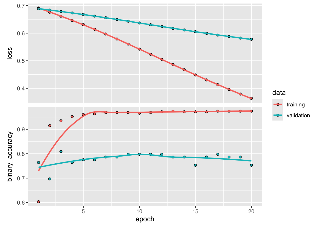

ImportantAction

Compute predictions from your trained network on the test partition. Estimate the predictive accuracy. Is it any better than what we managed with principal component regression in class?